Interrupted time series (ITS) designs are among the strongest quasi-experimental approaches available when randomized trials are infeasible, unethical, or impractical. They are widely used in epidemiology, public health, economics, and policy evaluation to estimate the causal effect of an intervention introduced at a specific point in time. Rather than comparing treated and untreated individuals, ITS compares outcomes within the same population before and after an intervention. By modeling outcome trends over time, researchers can detect whether a policy or intervention is associated with a sudden level change, a slope change, or both.
The major strength of ITS lies in its ability to control for stable confounders. Because the comparison is within the same population, it can be assumed that baseline characteristics largely do not change over time. ITS is therefore particularly attractive for evaluating population-level policies such as smoking bans, mass vaccination, or new clinical guidelines. When well specified, it can provide compelling evidence of causal effects even without individual-level treatment assignment.
However, ITS relies on several core assumptions. First, the pre-intervention trend must represent a valid counterfactual for what would have happened in the absence of the intervention. This assumption is fundamentally untestable, but its plausibility can be evaluated using theory, prior evidence, and diagnostic plots. Second, no other events occurring at the same time as the intervention should affect the outcome. If a second policy or external shock coincides with the intervention, disentangling their effects becomes difficult. Third, the functional form of the time trend must be correctly specified; mis-specifying seasonality or nonlinear trends can bias effect estimates. A Fourth, consistency of measurement: outcome definitions, surveillance systems, or reporting practices should not change overtime.
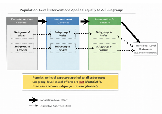
When these assumptions hold, ITS can estimate the causal effect of an intervention on the overall population. However, the method’s strength at the population level does not automatically extend to subgroup analyses. In fact, when interventions are implemented uniformly across all individuals, subgroup causal inference is not just difficult but fundamentally impossible. This is due to lack of identifiability.
Formally, for subgroup g:
Β(g)=E[Y(1)-Y(0)|G=g)
However, if treatment is uniform or equal across subgroups, then either everyone is treated or no one is treated. So one of these is never observed: Y(1) only or Y(0) only. Therefore, the causal contrast for that subgroup is not identifiable. For subgroup causal effects to be identifiable, at least one of the following sources of variation must exist: variation across time, variation across place, and variation in intensity/dose.
Population-level interventions frequently violate these requirements. Consider a national immunisation introduced on a single date and applied uniformly across all regions, sexes, and age groups. In such a case, there is no cross-group variation in exposure: everyone is treated simultaneously and equally. The intervention indicator is identical for all subgroups at every time point. Because subgroup membership does not influence treatment assignment, there is no contrast within time to estimate subgroup-specific effects.
Descriptive Subgroup Analysis as alternative to causal subgroup analysis
Although causal subgroup effects may be unidentified, descriptive subgroup analyses remain informative when interpreted correctly. Researchers can still estimate how outcomes changed over time within each subgroup and compare those changes. However, note that such analyses answer “Who changed more?” not “For whom did the policy work?”. This distinction is crucial. The first question is descriptive; it summarises observed patterns. The second is causal; it attributes differences to the intervention. Confusing the two leads to overinterpretation and potentially misleading conclusions.
For instance, let’s imagine that disease incidence falls more sharply among females than males after a national policy. A descriptive statement would be: “Incidence declined more among females than males following the policy.” A causal claim would be: “The policy was more effective for females than males.” The latter requires evidence that the difference would not have occurred without the intervention. Without variation in exposure, that claim is unsupported. The observed difference could reflect preexisting trends, differential measurement error, or unrelated subgroup-specific factors.
This distinction matters for policy decisions. Misinterpreting descriptive subgroup differences as causal heterogeneity can lead policymakers to believe an intervention benefits some groups more than others, potentially shaping resource allocation or future interventions based on flawed evidence. Researchers should therefore clearly label subgroup analyses from uniform population interventions.
References
- Pearl J. Causality: Models, Reasoning and Inference. Cambridge University Press, 2009.
- Imbens GW, Rubin DB. Causal Inference for Statistics, Social, and Biomedical Sciences. Cambridge University Press, 2015.
- Morgan SL, Winship C. Counterfactuals and Causal Inference. Cambridge University Press, 2015.
- Bernal JL, Cummins S, Gasparrini A. Interrupted time series regression for the evaluation of public health interventions. Int J Epidemiol. 2017.